41 display data labels in excel
How to add data labels in excel to graph or chart (Step-by-Step) 1. Select a data series or a graph. After picking the series, click the data point you want to label. 2. Click Add Chart Element Chart Elements button > Data Labels in the upper right corner, close to the chart. 3. Click the arrow and select an option to modify the location. 4. stacked column chart for two data sets - Excel - Stack Overflow Feb 01, 2018 · If you don't want to display all the months you can click on the labels of the months you don't want and it will disapear, like so: Once you have build your chart you can load it in Excel by using an excel add-in called Funfun.You just have to paste the URL of the online editor in the add-in. Here is how it looks like with my example:
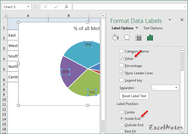
How to Display Percentage in an Excel Graph (3 Methods) Display Percentage in Graph. Select the Helper columns and click on the plus icon. Then go to the More Options via the right arrow beside the Data Labels. Select Chart on the Format Data Labels dialog box. Uncheck the Value option. Check the Value From Cells option.

Display data labels in excel
How to hide zero data labels in chart in Excel? - ExtendOffice 1. Right click at one of the data labels, and select Format Data Labels from the context menu. See screenshot: 2. In the Format Data Labels dialog, Click Number in left pane, then select Custom from the Category list box, and type #"" into the Format Code text box, and click Add button to add it to Type list box. See screenshot: 3. Custom Chart Data Labels In Excel With Formulas - How To Excel At Excel Follow the steps below to create the custom data labels. Select the chart label you want to change. In the formula-bar hit = (equals), select the cell reference containing your chart label's data. In this case, the first label is in cell E2. Finally, repeat for all your chart laebls. How to add data labels from different column in an Excel chart? This method will introduce a solution to add all data labels from a different column in an Excel chart at the same time. Please do as follows: 1. Right click the data series in the chart, and select Add Data Labels > Add Data Labels from the context menu to add data labels. 2.
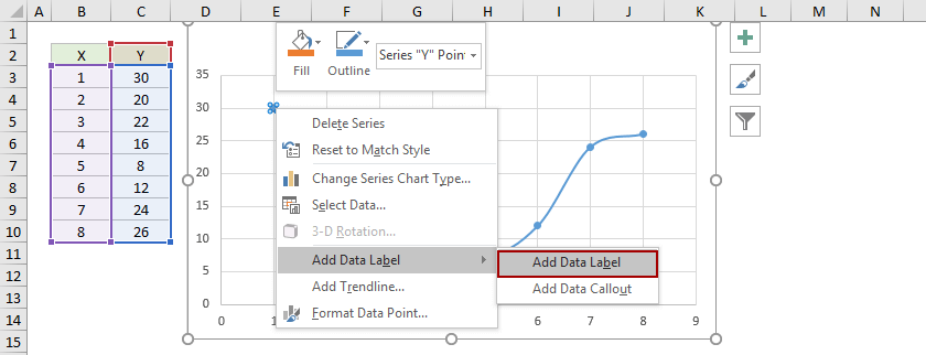
Display data labels in excel. How to Make Charts and Graphs in Excel | Smartsheet Jan 22, 2018 · To generate a chart or graph in Excel, you must first provide the program with the data you want to display. Follow the steps below to learn how to chart data in Excel 2016. Step 1: Enter Data into a Worksheet. Open Excel and select New Workbook. Enter the data you want to use to create a graph or chart. How To Plot X Vs Y Data Points In Excel | Excelchat Figure 6 – Plot chart in Excel. If we add Axis titles to the horizontal and vertical axis, we may have this; Figure 7 – Plotting in Excel. Add Data Labels to X and Y Plot. We can also add Data Labels to our plot. These data labels can give us a clear idea of each data point without having to reference our data table. We can click on the ... How do you display the data labels on this chart above the data markers ... Add data labels Click the chart, and then click the Chart Design tab. Click Add Chart Element and select Data Labels, and then select a location for the data label option. Note: The options will differ depending on your chart type. If you want to show your data label inside a text bubble shape, click Data Callout. Tutorial: Import Data into Excel, and Create a Data Model Note: Notice the checkbox at the bottom of the window that allows you to Add this data to the Data Model, shown in the following screen.A Data Model is created automatically when you import or work with two or more tables simultaneously. A Data Model integrates the tables, enabling extensive analysis using PivotTables, Power Pivot, and Power View.
5 Ways to Concatenate Data with a Line Break in Excel Sep 15, 2022 · The cell will now display on multiple lines. Conclusions. Excel has many options to combine data into a single cell with each item of data on its own line. Most of the time using a formula based solution will be the quickest and easiest way. We may find ourselves in need of an option which can’t easily be accidentally changed. How to add a line in Excel graph: average line, benchmark, etc. Select the last data point on the line and add a data label to it as discussed in the previous tip. Click on the label to select it, then click inside the label box, delete the existing value and type your text: Hover over the label box until your mouse pointer changes to a four-sided arrow, and then drag the label slightly above the line: How to add data labels from different column in an Excel chart? Right click the data series in the chart, and select Add Data Labels > Add Data Labels from the context menu to add data labels. 2. Click any data label to select all data labels, and then click the specified data label to select it only in the chart. 3. How to use data labels in a chart - YouTube Excel charts have a flexible system to display values called "data labels". Data labels are a classic example a "simple" Excel feature with a huge range of o...
Data labels on small states using Maps - Microsoft Community Data labels on small states using Maps. Hello, I need some assistance using the Filled Maps chart type in Excel (note: this is NOT Power Maps). I have some data (see attachment below) that I've plotted on a map of the USA. Because the data only applied to 7 states I changed the "map area" (under Format Data Series-->Series Options) to show ... Data Labels in Excel Pivot Chart (Detailed Analysis) 7 Suitable Examples with Data Labels in Excel Pivot Chart Considering All Factors 1. Adding Data Labels in Pivot Chart 2. Set Cell Values as Data Labels 3. Showing Percentages as Data Labels 4. Changing Appearance of Pivot Chart Labels 5. Changing Background of Data Labels 6. Dynamic Pivot Chart Data Labels with Slicers 7. Change the format of data labels in a chart To get there, after adding your data labels, select the data label to format, and then click Chart Elements > Data Labels > More Options. To go to the appropriate area, click one of the four icons ( Fill & Line, Effects, Size & Properties ( Layout & Properties in Outlook or Word), or Label Options) shown here. How to Add Data Labels in Excel - Excelchat | Excelchat In Excel 2013 and the later versions we need to do the followings; Click anywhere in the chart area to display the Chart Elements button Figure 5. Chart Elements Button Click the Chart Elements button > Select the Data Labels, then click the Arrow to choose the data labels position. Figure 6. How to Add Data Labels in Excel 2013 Figure 7.
Adding rich data labels to charts in Excel 2013 | Microsoft ...
Find, label and highlight a certain data point in Excel scatter graph Here's how: Click on the highlighted data point to select it. Click the Chart Elements button. Select the Data Labels box and choose where to position the label. By default, Excel shows one numeric value for the label, y value in our case. To display both x and y values, right-click the label, click Format Data Labels…, select the X Value and ...

Adding rich data labels to charts in Excel 2013 | Microsoft ...
Add or remove data labels in a chart - support.microsoft.com Right-click the data series or data label to display more data for, and then click Format Data Labels. Click Label Options and under Label Contains , select the Values From Cells checkbox. When the Data Label Range dialog box appears, go back to the spreadsheet and select the range for which you want the cell values to display as data labels.

How to make a pie chart in Excel
How to Add Data Labels to Scatter Plot in Excel (2 Easy Ways) - ExcelDemy By our previous action, a task pane named Format Data Labels opens. Firstly, click on the Label Options icon. In the Label Options, check the box of Value From Cells. Then, select the cells in the B5:B14 range in the Select Data Label Range box. These cells contain the Name of the individuals which we
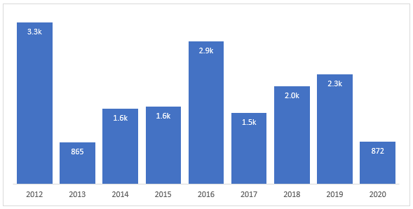
Format Chart Numbers as Thousands or Millions — Excel ...
How do you display category name and percentage data labels in Excel ... To format data labels, select your chart, and then in the Chart Design tab, click Add Chart Element > Data Labels > More Data Label Options. Click Label Options and under Label Contains, pick the options you want. To make data labels easier to read, you can move them inside the data points or even outside of the chart. How do you label a series ...

Change the format of data labels in a chart
Format Data Labels in Excel- Instructions - TeachUcomp, Inc. To format data labels in Excel, choose the set of data labels to format. To do this, click the "Format" tab within the "Chart Tools" contextual tab in the Ribbon. Then select the data labels to format from the "Chart Elements" drop-down in the "Current Selection" button group.

How To Show Or Hide Data Labels On MS Excel? | My Windows Hub
5 New Charts to Visually Display Data in Excel 2019 - dummies Aug 26, 2021 · Select the data and labels and then click Insert → Maps → Filled Map. Wait a few seconds for the map to load. Resize and format as desired. For example, you could apply one of the chart styles from the Chart Tools Design tab. To add data labels to the chart, choose Chart Tools Design → Add Chart Element → Data Labels → Show. Pouring ...

Apply Custom Data Labels to Charted Points - Peltier Tech
Excel tutorial: How to use data labels Generally, the easiest way to show data labels to use the chart elements menu. When you check the box, you'll see data labels appear in the chart. If you have more than one data series, you can select a series first, then turn on data labels for that series only. You can even select a single bar, and show just one data label.

Adding rich data labels to charts in Excel 2013 | Microsoft ...
Edit titles or data labels in a chart - support.microsoft.com The first click selects the data labels for the whole data series, and the second click selects the individual data label. Right-click the data label, and then click Format Data Label or Format Data Labels. Click Label Options if it's not selected, and then select the Reset Label Text check box. Top of Page

Apply Custom Data Labels to Charted Points - Peltier Tech
How To Add Data Labels In Excel - gr8idea.info Data labels are used to display source data in a chart directly. Change position of data labels. Source: . The column chart will appear. For example, this is how we can add labels to one of the data series in our excel chart: Source: . Click the + symbol and add data labels by clicking it as shown below step 3 ...

424 How to add data label to line chart in Excel 2016
data labels not showing all options - Microsoft Community Hi all, I am working on a graph in excel office 365. It's a histogram. Now I want the data label to display the category name, but the only options I see are "series name" and "value". Any ideas how

Adding rich data labels to charts in Excel 2013 | Microsoft ...
Adding Data Labels to Your Chart (Microsoft Excel) - ExcelTips (ribbon) To add data labels in Excel 2013 or later versions, follow these steps: Activate the chart by clicking on it, if necessary. Make sure the Design tab of the ribbon is displayed. (This will appear when the chart is selected.) Click the Add Chart Element drop-down list. Select the Data Labels tool.

Chart Data Labels in PowerPoint 2013 for Windows
Add or remove data labels in a chart - support.microsoft.com Right-click the data series or data label to display more data for, and then click Format Data Labels. Click Label Options and under Label Contains, select the Values From Cells checkbox. When the Data Label Range dialog box appears, go back to the spreadsheet and select the range for which you want the cell values to display as data labels.

Adding rich data labels to charts in Excel 2013 | Microsoft ...
How to display text labels in the X-axis of scatter chart in Excel? Select the data you use, and click Insert > Insert Line & Area Chart > Line with Markers to select a line chart. See screenshot: 2. Then right click on the line in the chart to select Format Data Series from the context menu. See screenshot: 3. In the Format Data Series pane, under Fill & Line tab, click Line to display the Line section, then ...

Adding rich data labels to charts in Excel 2013 | Microsoft ...
How to add data labels from different column in an Excel chart? This method will introduce a solution to add all data labels from a different column in an Excel chart at the same time. Please do as follows: 1. Right click the data series in the chart, and select Add Data Labels > Add Data Labels from the context menu to add data labels. 2.

How to Make Pie Chart with Labels both Inside and Outside ...
Custom Chart Data Labels In Excel With Formulas - How To Excel At Excel Follow the steps below to create the custom data labels. Select the chart label you want to change. In the formula-bar hit = (equals), select the cell reference containing your chart label's data. In this case, the first label is in cell E2. Finally, repeat for all your chart laebls.

Add or remove data labels in a chart
How to hide zero data labels in chart in Excel? - ExtendOffice 1. Right click at one of the data labels, and select Format Data Labels from the context menu. See screenshot: 2. In the Format Data Labels dialog, Click Number in left pane, then select Custom from the Category list box, and type #"" into the Format Code text box, and click Add button to add it to Type list box. See screenshot: 3.
![Fixed:] Excel Chart Is Not Showing All Data Labels (2 Solutions)](https://www.exceldemy.com/wp-content/uploads/2022/09/Showing-All-Data-Labels-Excel-Chart-Not-Showing-All-Data-Labels.png)
Fixed:] Excel Chart Is Not Showing All Data Labels (2 Solutions)

How to Change Excel Chart Data Labels to Custom Values?

Change the format of data labels in a chart

Format Number Options for Chart Data Labels in Excel 2011 for Mac

Apply Custom Data Labels to Charted Points - Peltier Tech

Change the format of data labels in a chart
![Fixed:] Excel Chart Is Not Showing All Data Labels (2 Solutions)](https://www.exceldemy.com/wp-content/uploads/2022/09/Selecting-Data-Callout-Excel-Chart-Not-Showing-All-Data-Labels.png)
Fixed:] Excel Chart Is Not Showing All Data Labels (2 Solutions)

How to Add Axis Labels to a Chart in Excel | CustomGuide

Quick Tip: Excel 2013 offers flexible data labels | TechRepublic

Dynamic Number Format for Millions and Thousands - PK: An ...

How to Add Data Labels to your Excel Chart in Excel 2013
![Fixed:] Excel Chart Is Not Showing All Data Labels (2 Solutions)](https://www.exceldemy.com/wp-content/uploads/2022/09/Data-Label-Reference-Excel-Chart-Not-Showing-All-Data-Labels.png)
Fixed:] Excel Chart Is Not Showing All Data Labels (2 Solutions)
How to Make Pie Chart with Labels both Inside and Outside ...
How to add data labels from different column in an Excel chart?
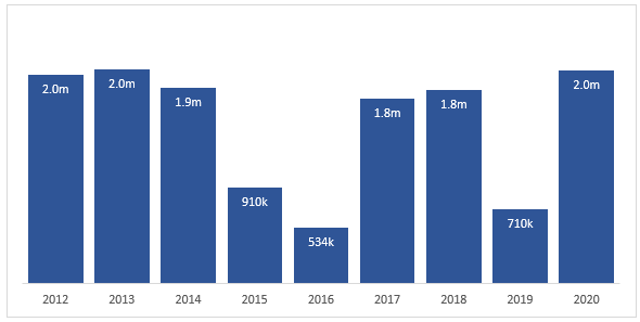
Format Chart Numbers as Thousands or Millions — Excel ...

How-to Use Data Labels from a Range in an Excel Chart - Excel ...

Enable or Disable Excel Data Labels at the click of a button ...

Format Number Options for Chart Data Labels in PowerPoint ...

Change the format of data labels in a chart
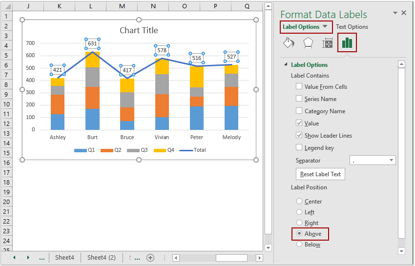
How to add total labels to stacked column chart in Excel?

Excel Charts - Aesthetic Data Labels

Excel Charts: Dynamic Label positioning of line series

Creating Pie Chart and Adding/Formatting Data Labels (Excel)

How to show percentages on three different charts in Excel ...
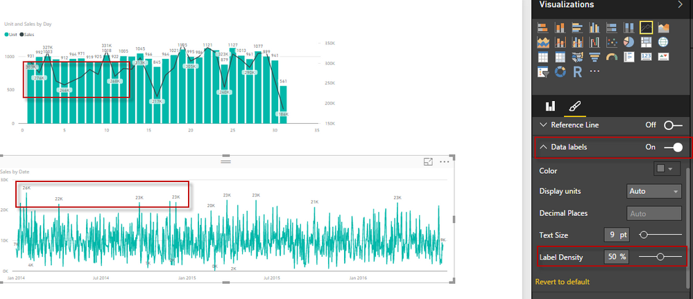
Solved: Data Labels - Microsoft Power BI Community
Post a Comment for "41 display data labels in excel"